Your preparation for the lab session
Why does the chair spring back?
A cantilever chair supports you without rear legs beneath the seat. Its bent tubes deform under your weight.
Load and unload the chair model. As long as deformation remains elastic, the frame springs back.
Observe how much the chair deforms under load. The following sections explain the differences between stiffness, strength and ductility.
Stiffness, strength and ductility
What do you expect when replacing steel with aluminium? Try different materials in the beam model. Keep the tube dimensions and load unchanged for your first comparison.
- Stiffness
- How much does the component deform under a load?
- Strength
- How high can the stress become before permanent deformation or failure begins?
- Ductility
- How far can a material deform permanently before it fractures?
A higher-strength steel is not necessarily stiffer. The deformation of the chair depends on both the material and the tube dimensions.
Specimen and testing machine
Both material and shape affect how the chair deforms. In a tensile test, you test a specimen with known dimensions to determine the properties of the material.
The specimen is gripped at both ends and pulled apart by the tensile force \(F\). To analyse a round specimen, you need its initial diameter \(d_0\) and original gauge length \(L_0\).
The gauge length is the section of the specimen over which extension is measured. It is shorter than the specimen as a whole.
Measuring force and extension
The testing machine records the force F and the extension ΔL. Select Play to watch the measurement curve develop. Select Pause to stop playback. Drag the slider forwards or backwards to view a particular point in the test. Play resumes from that position.
The gauge length increases from \(L_0\) to \(L_0 + \Delta L\). \(\Delta L\) is the increase, not the full current gauge length.
The specimen first deforms elastically. Permanent deformation follows. After the maximum force, the specimen necks and eventually fractures.
Force and extension also depend on the specimen dimensions. Stress and strain are calculated from these measurements so that materials can be compared.
Stress and strain
At the same strain, a long specimen extends more than a short one. To calculate strain \(\varepsilon\), divide the extension \(\Delta L\) by the original gauge length \(L_0\).
Engineering stress σ = F / S₀
Strain ε = ΔL / L₀
S₀ is the initial cross-sectional area. For a round specimen, S₀ = π · d₀² / 4. With F in N and S₀ in mm², stress is in N/mm², which equals MPa. Strain is a dimensionless ratio; multiply it by 100 to obtain a percentage.
Switch between the two plots. The normalised curves coincide up to the maximum stress. They differ during necking: elongation after fracture depends on specimen geometry.
Determining material properties
The stress–strain curve provides measures of stiffness, strength and ductility:
- Young’s modulus E
- The slope of the straight elastic section describes the elastic stiffness of the material.
- yield strength Rₑ
- It marks the onset of appreciable plastic deformation. Here, the marker indicates the upper yield strength of structural steel S235.
- Ultimate tensile strength Rₘ
- It is the maximum engineering stress in the test. The force reaches its maximum here; necking then begins.
- Elongation after fracture A
- It is the permanent strain after fracture and a measure of ductility. The dashed line subtracts the elastic part of the total strain to provide an estimate.
For materials without a distinct yield point, the 0.2% proof strength \(R_{p0.2}\) is determined instead. The further reading explains this distinction.
Elastic region E = Δσ / Δε
Young’s modulus and yield strength help explain the deformation and elastic load capacity of the chair model. You will determine these properties in the virtual test.
Run and evaluate virtual tensile tests
Complete the following five tests and evaluate the curves. Structural steel S235 is required. Choose the second material yourself.
- Compare materialsS235 and your chosen material
- Investigating scatterThree short S235 specimens
- Investigating the effect of gauge lengthOne long S235 specimen
Your diagrams and observations become your preparation report. Download the PDF and bring it to the laboratory.
1 What is this about?
Virtually no object in our universe is free from mechanical loading: forces act everywhere. They deform the objects they act on and, if they become too large, permanently damage or destroy them.
- On the largest scale: the Earth is not a perfect sphere, because the centrifugal forces of its rotation flatten it into an oblate spheroid.
- In our bodies: walking, running and sport can subject muscles, tendons and bones to extreme loads, sometimes resulting in torn muscle fibres or broken bones.
- In nature: snow loads and storms bend tree branches considerably; some branches break, and sometimes even the trunk does.
- In everything we make: a smartphone falling to the ground, a car hitting a pothole, or a machine producing components day after day.
Engineers have therefore developed a set of methods for assessing how heavily an object is loaded and whether it can withstand that loading over time. These methods are universal: the same approach can be used to assess a thigh bone, a snow-covered branch, a smartphone housing or an overhead crane bridge.
In mechanical engineering, these methods are used during development: long before a product is built, it should be clear that it will function reliably throughout its service life. The properties of its structural material play a central role.
GlossaryKey words & Abbreviations
- Tensile test
- Uniaxial test to determine deformation and fracture behavior.
- DIN EN ISO 6892-1
- Test standard for the tensile test on metallic materials at room temperature.
- material property
- Geometry-independent, comparable material property (e.g. E, Rm).
- quasi-static
- Slow, shock-free loading without significant strain rate effects.
- ductile/brittle
- High or low plastic deformability up to fracture.
2 Stiffness, strength, ductility: from component to material
An everyday product illustrates which material properties matter in design: a cantilever chair.
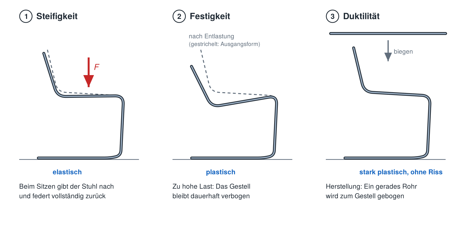
- Stiffness. When you sit on a chair, it deflects slightly and springs back completely when you stand up. This deformation is elastic. Stiffness describes its magnitude: an excessively flexible chair feels unstable and bouncy even if it does not break. For many technical components, this is the decisive criterion, for example a machine-tool frame that must barely deform.
- Strength. If someone drops heavily into the chair or stands on it, the frame may remain bent: the deformation is now plastic. Under an even greater load, it breaks. Strength describes the loading that can be sustained before permanent deformation or failure occurs.
- Ductility. The frame is bent from a straight steel tube; in some designs, the seat shell is pressed from flat sheet metal. This deliberately causes substantial plastic deformation, yet the material must not crack. This ability to deform is called ductility. It matters for manufacturing, for example deep drawing car-body panels or drinks cans, and for safety: a ductile component visibly bends before breaking, providing warning of failure. A car's crumple zone uses this behaviour to absorb impact energy through plastic deformation.
A component's stiffness and strength depend on two things: its geometry and its material. A thicker tube is stiffer and stronger than a thinner tube of the same material. Conversely, a chair with exactly the same tube dimensions but made of aluminium instead of steel would deflect about three times as much under the same load.
Try it: a beam model of the cantilever chair
How stiff and how strong is a cantilever chair, and what role does the material play? The application represents one side of the chair as a beam model: the curved steel tube is replaced by its centreline and calculated as a frame of bending beams. These are the same tools you know from engineering mechanics (strength of materials): bending moment, second moment of area I and section modulus W of the tube cross-section.
Adjust the material, tube outer diameter and wall thickness, body mass, leaning force and the option to sit down heavily. The magnification factor makes the deformation visible, which would otherwise be only a few millimetres.
- Seat deflection: It shows how stiff the chair is.
- Frame colour: It shows the stress in the tube relative to what the material can withstand without permanent deformation. Green means a large reserve; red means the limit for permanent deformation has been exceeded. This illustrates strength.
The application uses quantities introduced in later sections: the stress in the tube (Section 5), Young's modulus E and the yield strength (Section 6). These are precisely the material properties supplied by a tensile test. Without them, neither the chair's deformation nor its load capacity could be calculated.
Prepared experiments
Model details and values to revisit after Section 6
Each side frame consists of Euler–Bernoulli beam elements, with a pin support at the rear and a roller support at the front. The calculation includes axial force and bending for small deformations; it excludes transverse shear deformation and plastic deformation.
Above the material limit, the colour indicates the limit of the elastic calculation. It does not predict permanent deformation or fracture. The material properties are example values for this teaching model.
The model assumes that tube bends retain their circular cross-section. Real thin-walled tube bends can flatten and therefore deflect more. Contact between the entire base and the floor is also excluded.
Observe and compare
Start with the prepared experiments and consider these questions:
- What changes when you replace steel with aluminium, and what stays the same?
- What happens when you sit down heavily?
- How must you change the tube to make an aluminium chair as stiff as a steel chair, and how much does it then weigh?
Return to this model after Section 6. Use the material properties to explain the differences between the settings.
Stiffness and strength are independent properties: with the same geometry, a higher-strength steel can show the same elastic deformation as structural steel while withstanding a greater load without permanent deformation.
Exercise: Which statement is true?
Two components with identical geometry are subjected to the same force in the elastic range. Component A is steel, component B is aluminium. Use your observations from the beam model. Which statement is right?
GlossaryKey words & Abbreviations
- Stiffness
- A component's resistance to elastic deformation; depends on its material and geometry.
- Strength
- Resistance to permanent deformation and failure.
3 The tensile test: specimen and testing machine
The tensile test determines a material's mechanical properties using a specimen that is pulled slowly, without shocks (quasi-statically), until it fractures. Specimen shape, test procedure and evaluation are standardised, for metals at room temperature in DIN EN ISO 6892-1, so that results from different testing laboratories can be compared.
The specimen
The standard permits several specimen geometries, particularly round and flat specimens of different dimensions. They share two gripping sections with a larger cross-section and a gauge section with a smaller cross-section between them, connected by gently rounded transitions. The smaller cross-section ensures that the material is most heavily loaded in the gauge section: this is where it deforms and fractures, rather than at the grips, where clamping introduces additional, uneven loading.
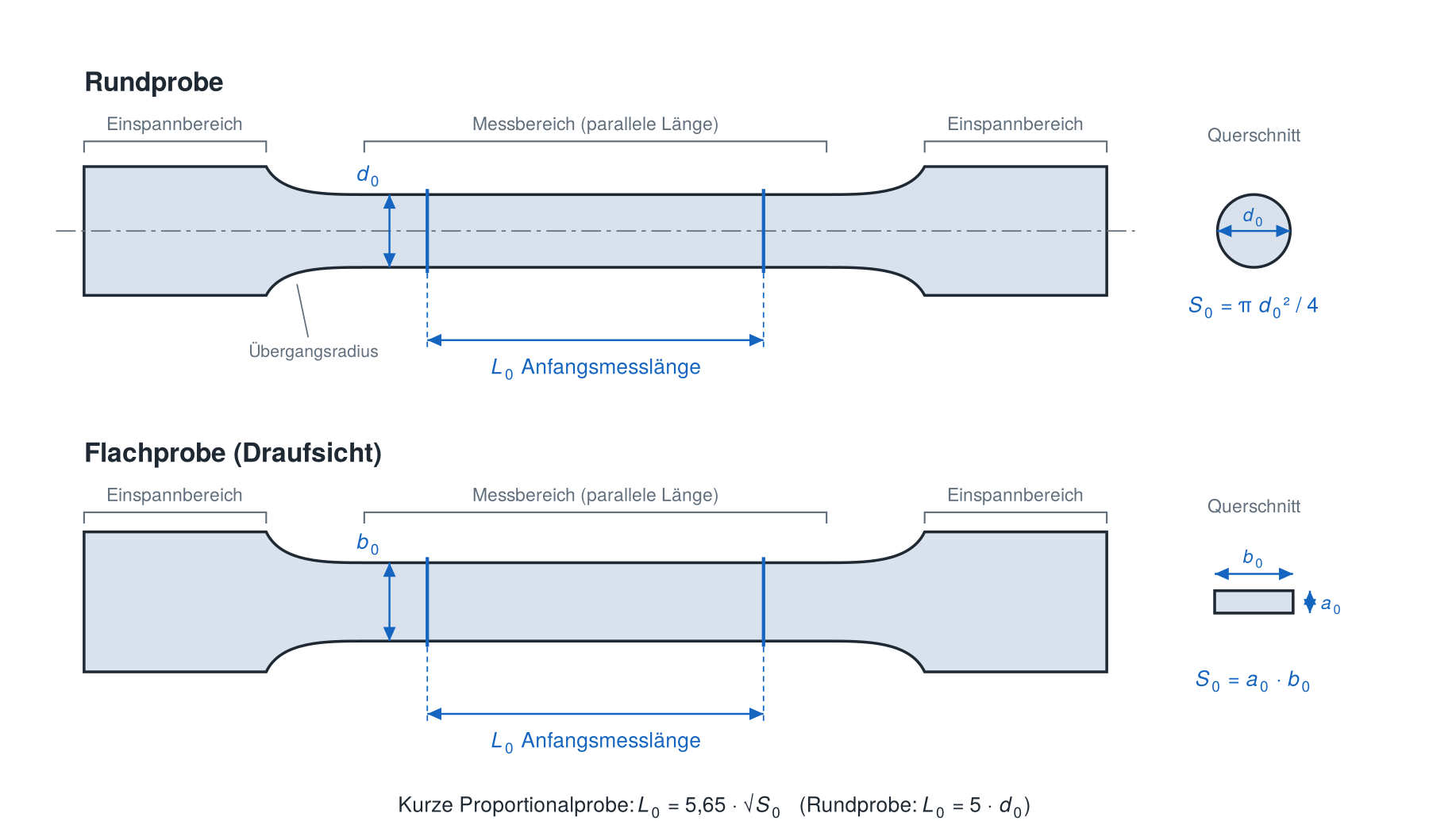
Before testing, two quantities used in the evaluation are carefully determined:
- the initial gauge length \(L_0\), over which elongation is measured,
- the initial cross-section \(S_0\), calculated from diameter \(d_0\) for round specimens and from width \(b_0\) and thickness \(a_0\) for flat specimens.
For comparable elongation after fracture, the standard requires a fixed relationship between gauge length and cross-section. Such specimens are called proportional specimens (section 6 explains why this matters):
DIN 50125 specifies standard geometries, for example form \(A\) (round specimen with plain ends), form B (round specimen with threaded ends) and form \(E\) (flat specimen with heads).
The testing machine
The specimen is clamped in a tensile testing machine.
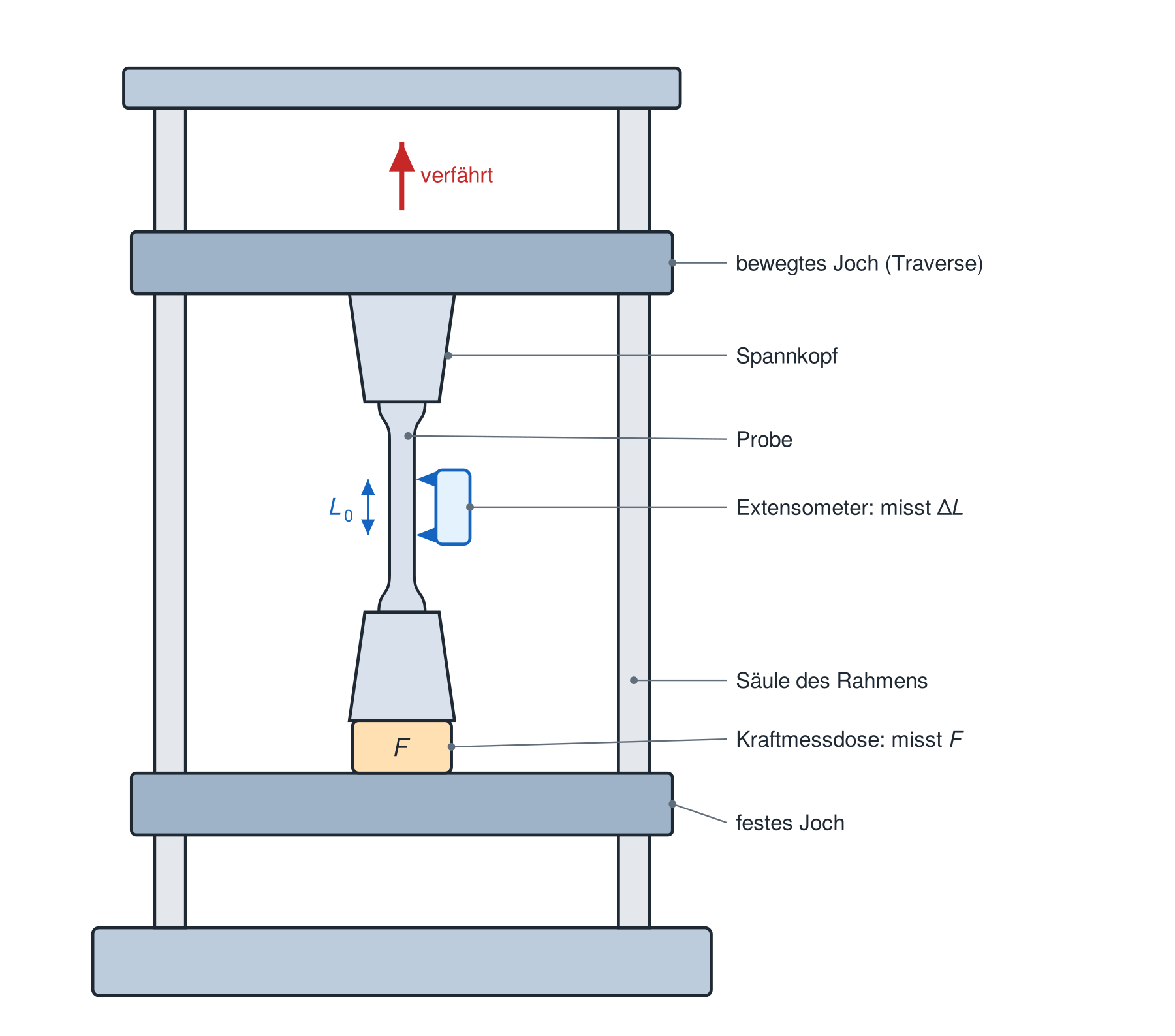
One crosshead is fixed; the other moves away slowly and steadily, extending the specimen until it fractures. Two quantities are recorded continuously:
- force \(F\), using a load cell,
- elongation \(\Delta L\) in the gauge section, using an extensometer with knife edges in direct contact with the specimen, or a contactless camera system (video extensometry or digital image correlation).
The extensometer measures much more accurately than crosshead travel, because crosshead travel also includes the compliance of the grips and machine frame.
Standards at a glance: DIN EN ISO 6892-1 (tensile testing of metals at room temperature) · DIN EN ISO 6892-2 (elevated temperature) · DIN 50125 (specimen shapes) · DIN EN ISO 527 (plastics) · ASTM E8/E8M (US standard for metals).
GlossaryKey words & Abbreviations
- F
- Force / N — recorded via the load cell.
- ΔL
- Change in length / mm — recorded via the extensometer.
- L0
- Initial gauge length — reference length used to calculate strain.
- S0
- Initial cross-sectional area — reference area used to calculate stress.
- d0
- Specimen diameter (round specimen).
- Extensometer
- Length measuring system via L0; more accurate than crosshead-displacement measurement.
- Load cell
- Sensor for measurement of the test force F.
- Proportional specimen
- Fixed ratio specimen L0 = 5,65·√S0.
- DIN 50125
- Standard for geometrically defined tensile specimens.
4 Primary measurements: the force–elongation curve
The primary measurements in tensile testing are force \(F\) and elongation \(\Delta L\). Plotting them produces the force–elongation diagram.
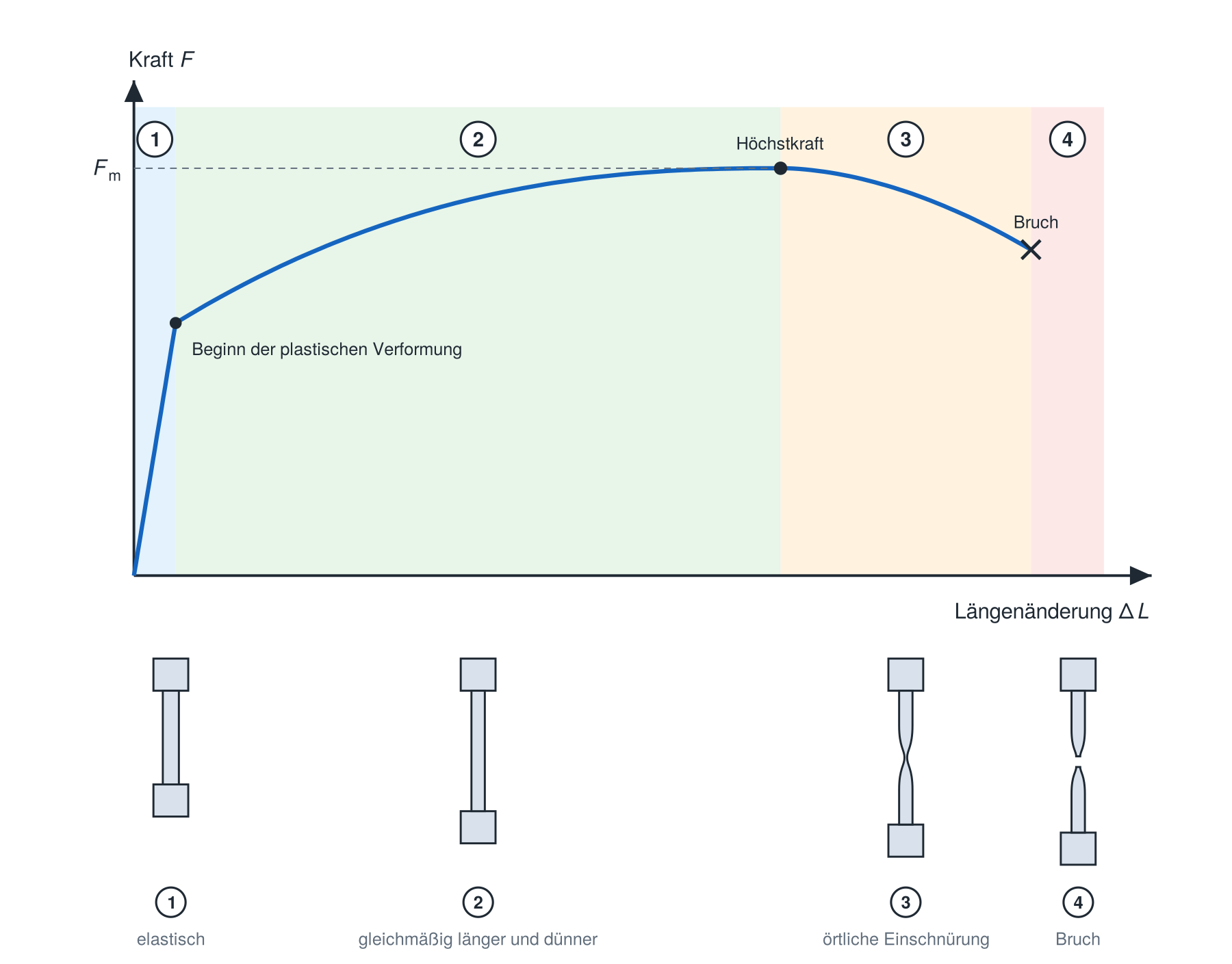
The curve shows what happens to the specimen:
- Elastic deformation. Force increases linearly. When unloaded, the specimen returns completely to its original shape.
- Plastic deformation with strain hardening. Above a certain force, permanent deformation begins: dislocations glide in the crystal lattice. Force now increases more gradually because dislocations hinder one another and the material strain-hardens. The specimen becomes uniformly longer and thinner throughout the gauge length.
- Necking. At maximum force \(F_m\), strain hardening can no longer compensate for the continuous reduction in cross-section. Deformation concentrates at one location, producing a clearly visible neck. From this point, further extension requires progressively less force.
- Fracture. Microscopic voids form and coalesce in the neck until the specimen fractures, producing the typical cup-and-cone fracture surface in ductile metals.
The drop in force after \(F_m\) therefore does not mean that the material becomes weaker: deformation becomes geometrically unstable, and the cross-section at the neck decreases faster than strain hardening can compensate for.
Effect of specimen geometry
The force–extension curve depends on the specimen geometry as well as the material. A thicker specimen of the same material carries a higher force, while a longer specimen extends further under the same loading conditions. As with the chair frame in Section 2, the curve describes the whole component rather than the material alone. Try changing the dimensions below:
Specimen 1
Specimen 2 — with other parameters
Choose the same material, but one different geometry (different diameter and/or different gauge length). Then observe how the curves differ.
Force–extension diagram
5 Secondary quantities: stress and strain
To obtain the material behaviour alone, the primary measurements are related to specimen geometry. It is not force alone that determines the loading of the material, but how that force is distributed across the cross-section. Engineering stress is therefore introduced as force divided by the initial cross-section:
This simple calculation is valid because the gauge section has a uniform, uniaxial stress state. Stress measures the loading of the material: under the same force, the material in a thick specimen is less heavily loaded than in a thin one.
Similarly, engineering strain is elongation divided by the initial gauge length:
It measures material deformation independently of the gauge length. The primary measurements thus become secondary quantities, producing the characteristic stress–strain curve of the material. Repeat the two tests above, this time in the \(\sigma\)-\(\varepsilon\) diagram:
The curves are calculated using a material model, without scatter or measurement noise. The default specimens have the same diameter and different gauge lengths, making the effect of necking visible.
Specimen 1 — this time in -
Specimen 2 - this time in -
Stress–strain diagram
Up to the maximum stress, the curves for the same material coincide. Beyond that point, the curve depends on specimen geometry: specimens with the same diameter and different gauge lengths have different curves during necking. Proportionally scaled specimens can still have the same curve beyond the maximum. Section 6 explains the connection with elongation after fracture.
Engineering stress and true stress
\(S_0\) and \(L_0\) are initial values and are not updated during the test; hence the term engineering. In reality, the specimen becomes thinner as it is pulled. True stress, based on the current cross-section, is therefore always greater than engineering stress and continues to rise after \(F_m\). Engineering stress falls during necking solely because it refers to the original cross-section. Standardised properties consistently use engineering quantities.
Regions of the \(\sigma\)-\(\varepsilon\) curve
The stages described in section 4 also appear in the \(\sigma\)-\(\varepsilon\) curve. Select a material and click on the regions:
Elastic deformation
Force increases linearly. When unloaded, the specimen returns completely to its original shape.
Plastic deformation with strain hardening
Above a certain force, permanent deformation begins: dislocations glide in the crystal lattice. Force now increases more gradually because dislocations hinder one another and the material strain-hardens. The specimen becomes uniformly longer and thinner throughout the gauge length.
Necking
At maximum force \(F_m\), strain hardening can no longer compensate for the continuous reduction in cross-section. Deformation concentrates at one location, producing a clearly visible neck. From this point, further extension requires progressively less force.
Fracture
Microscopic voids form and coalesce in the neck until the specimen fractures, producing the typical cup-and-cone fracture surface in ductile metals.
Exercise: Calculate stress
A force of \(F = 30\,000\,\mathrm{N}\) is measured on a round specimen with an initial diameter of \(d_0 = 10\,\mathrm{mm}\). Calculate the engineering stress in MPa.
Enter decimals using a comma or a point.
Exercise: Which diagram stays the same?
You test two round S235 specimens with different initial diameters: \(d_0 = 5\,\mathrm{mm}\) and \(d_0 = 10\,\mathrm{mm}\). In which diagram do the curves coincide up to the maximum stress?
Exercise: Assign phases
Match each description with the correct phase.
1. Deformation disappears completely after unloading
2. The cross-section becomes smaller locally and the engineering stress appears to decrease
3. Permanent deformation with increasing stress to the maximum point
GlossaryKey words & Abbreviations
- Primary data
- Directly measured, geometry-dependent variables F and ΔL.
- Secondary data
- Quantities referred to the initial geometry and .
- Engineering stress / MPa = F / S0.
- Technical elongation / — = ΔL / L0.
- Standardization
- Reference to the measured quantities S0 and. L0.
- technical/true
- Reference to the initial (technical) or current cross-section (true).
- elastic
- The deformation disappears completely after unloading.
- plastic
- Area of permanent (non-reversible) deformation.
- Translation
- Line defect in the crystal lattice, the sliding of which supports the plastic deformation.
- strain hardening
- Increase in strength through mutual blocking of the dislocations.
- Lüders-Plateau
- Yielding region at approximately constant stress.
- Necking
- Local reduction in cross-section after reaching the maximum stress.
- Fracture
- Failure of the specimen in the necking area.
- Ductility
- Capacity for plastic deformation before fracture.
6 Material properties according to DIN EN ISO 6892-1
The \(\sigma\)-\(\varepsilon\) curve provides the properties describing stiffness, strength and ductility. Select a material; clicking a marker highlights the corresponding explanation.
Young's modulus \(E\) – stiffness
Young's modulus is the slope of the curve in the linear-elastic region and is determined by linear regression over that region:
For a given material, \(E\) is almost independent of heat treatment or degree of cold working. Typical values: steel ≈ 200 to 210 GPa, titanium ≈ 105 to 115 GPa, copper ≈ 110 to 125 GPa, aluminium ≈ 69 to 72 GPa.
Yield strength – onset of plastic deformation
Depending on the material, the transition from elastic to plastic behaviour appears in two ways:
- A distinct yield point, typical of unalloyed structural steels such as S235: stress drops markedly at the onset of yielding and then remains on an almost horizontal Lüders plateau while dull yield markings travel along the specimen. The upper yield strength \(R_{\mathrm{eH}}\) (highest stress before the first drop) and lower yield strength \(R_{\mathrm{eL}}\) (lowest stress during yielding, disregarding initial transient effects) are determined.
- A gradual transition, typical of quenched and tempered steels, austenitic steels and aluminium alloys: no clear onset of yielding is visible. Instead, the proof strength \(R_{\mathrm{p0,2}}\) is constructed: the stress that would leave a permanent strain of 0.2 % after unloading. The elastic line is shifted horizontally to the right by \(\varepsilon\) = 0.002; its intersection with the curve gives \(R_{\mathrm{p0,2}}\).
Tensile strength \(R_m\) – highest sustained stress
Tensile strength is the highest engineering stress in the test, reached at maximum force:
Uniform elongation \(A_g\)
This is the plastic strain at maximum force, before necking begins. It describes how far the material can deform uniformly over the entire gauge length. Graphically, it is the strain-axis intercept of a line parallel to the elastic line passing through the \(R_m\) point.
Elongation after fracture \(A\) – ductility
Elongation after fracture is the permanent strain remaining after fracture and the main measure of ductility. It is determined by fitting the two fractured pieces together and measuring the final gauge length \(L_u\):
If the extensometer remains attached until fracture, \(A\) may also be determined graphically, similarly to \(A_g\), using a parallel line through the fracture point. Because \(A\) includes the deformation within the neck, \(A\) > \(A_g\) always holds.
Which properties depend on the specimen?
\(E\), yield strength, \(R_m\) and \(A_g\) are determined while the specimen still deforms uniformly over its entire gauge length. They are therefore largely independent of specimen geometry.
Elongation after fracture is different: it includes the additional extension within the neck. The neck extends over roughly one to two specimen diameters; its contribution to elongation therefore increases with specimen thickness but is independent of gauge length. Relative to a short gauge length, this fixed contribution has a greater effect than relative to a long one: the shorter the gauge length in relation to cross-section, the greater the elongation after fracture. The Oliver relationship describes this approximately:
This is why proportional specimens are used (section 3), and why elongation after fracture is always stated together with specimen geometry: \(A\) for the short proportional specimen (\(L_0\) = 5,65·√\(S_0\), for round specimens \(L_0\) = 5·\(d_0\)), \(A_{11,3}\) for the long one (\(L_0\) = 11,3·√\(S_0\), for round specimens \(L_0\) = 10·\(d_0\)). Older standards, many datasheets and textbooks still call these values \(A_5\) and \(A_{10}\); they refer to the same quantities. Try the comparison in section 5: keep the diameter constant and use substantially different gauge lengths.
Exercise: Calculate Young’s modulus
In the elastic region, a strain of \(\varepsilon = 0.001\) corresponds to a stress of \(\sigma = 210\,\mathrm{MPa}\). Calculate Young’s modulus in MPa.
Exercise: Match the material properties
Match each description to the correct material property.
1. Slope in the linear region of the curve
2. Highest engineering stress in the curve
3. Stress at 0.2% permanent elongation
GlossaryKey words & Abbreviations
- E
- Modulus of elasticity / GPa — slope in the elastic range (stiffness).
- ReH
- Upper yield strength — highest stress before the force drops.
- ReL
- Lower yield strength — lowest stress on the Lüders plateau.
- Rp0.2
- 0.2% proof strength (continuous yielding).
- Rm
- tensile strength / MPa — maximum engineering stress.
- Ag
- Uniform elongation — plastic elongation at maximum force.
- A
- elongation after fracture / % — permanent elongation after fracture (ductility).
- 0.2% offset
- A line parallel to the elastic line at \(\varepsilon = 0.002\), used to determine the proof strength \(R_{\mathrm{p0.2}}\).
7 The virtual tensile test: preparing for the laboratory
Your preparation for the materials laboratory
Run and evaluate virtual tensile tests
You will carry out five tensile tests using two materials. Structural steel S235 is required. Choose one of the other three materials as your second material. Compare the materials and investigate variability and the effect of gauge length.
Your plots and observations are collected in the preparation report. Bring the PDF to the lab session.
Review the fundamentals: Sections 1–6Preparing for the tests
The curves are calculated using a material model. It describes elastic and permanent deformation, necking and fracture. Elongation after fracture also depends on specimen geometry.
Keep measurement noise and scatter enabled. Measurement noise causes small fluctuations in the readings, while variability causes differences between specimens of the same material. You will investigate these effects in the repeat tests.
First test S235 and your second material with d₀ = 10 mm and L₀ = 50 mm. Repeat the S235 test twice. Finally, test an S235 specimen with L₀ = 100 mm. After each evaluation, select “Accept results” and record your observations.
Read more about the model and materials
Read the following preparation before choosing your materials and starting the first test. It explains the model, the available materials and your tasks.
What is behind the virtual experiment?
No real specimens are tested here. A material model calculates the curves and describes material behaviour mathematically. It reproduces the stages introduced in the fundamentals:
- Elastic deformation: the specimen springs back after unloading. The slope of the stress–strain curve describes its elastic stiffness.
- Plastic deformation and strain hardening: the specimen deforms permanently. Further deformation initially requires more force. Depending on the material, yielding has either a distinct yield point or a gradual transition.
- Necking and fracture: deformation becomes concentrated in one region, the force drops and the specimen fractures. The model accounts for the dependence of measured elongation after fracture on specimen geometry.
The model also includes scatter and measurement noise. Scatter means that two specimens of the same material have slightly different properties. Measurement noise means that the measured values fluctuate slightly. Leave both options enabled for this test programme: observing these differences is the purpose of the repeat tests.
The simulation prepares you for the lab session. Compare the calculated material properties with the reference values. The results do not replace a test on a real specimen.
S235 is compulsory: an overview of the four materials
- Structural steel S235: a commonly used steel for load-bearing components. It is readily formable and shows a distinct yield point with a Lüders plateau in the model.
- CrNi steel 1.4301: a stainless steel, often called “V2A”. It has a gradual transition to yielding and can undergo substantial plastic deformation, for example in food-processing applications.
- Quenched and tempered steel 42CrMo4: a steel given high strength by heat treatment. Typical applications include shafts and gears.
- Aluminium alloy 7075: a lightweight, high-strength aluminium material used in lightweight structures. It is much more flexible elastically than steel.
Material A is always structural steel S235. For material B, choose CrNi steel 1.4301, quenched and tempered steel 42CrMo4 or aluminium alloy 7075. Use this combination throughout the test programme.
What you will do and submit
You will carry out five tests: a short specimen of A, a short specimen of B, two more short specimens of A and finally a long specimen of A. The repeat tests reveal the scatter. The long specimen lets you investigate the effect of gauge length.
Start each test directly within its task. Then determine the material properties and select “Accept results”. Your diagram appears in the text and is added to the report. Record your observation and proceed to the next task. Finally, export the five tests with their diagrams and observations as a PDF.
Choose the materials for your test series
Structural steel S235 is compulsory as material A for the evaluation. For material B, choose one of the other three materials. This choice becomes fixed for the assignment when you open the first test.
The requirement has changed: S235 is now compulsory. Previously saved results remain under “Test series”. Tasks that do not meet the requirement must be repeated using S235.
No tests completed yet.
Compare materials
1 · Test structural steel S235
Read before the test
How your measurement curve develops
Initially, the specimen deforms elastically: if unloaded, it would return to its original shape. Further stretching causes permanent deformation. After the maximum force, the specimen develops a neck and eventually fractures. You calculate stress and strain from force and elongation, then use them to determine the material properties.
Your task
Test a short round specimen of structural steel S235 to fracture. First observe the force and elongation. Then evaluate the curve and determine the material properties.
Material A · d₀ = 10 mm · L₀ = 50 mm
The material and specimen dimensions are preset for this task. Start the test and evaluate the curve. Then select “Accept results”. Your plot will appear below the task.
Record and explain your observations
Which regions can you identify in your curve? How does permanent deformation begin?
2 · Compare the second material with S235
Read before the test
Compare stiffness, strength and ductility
Young’s modulus describes elastic stiffness: the higher it is, the steeper the elastic line. Yield strength and tensile strength describe strength. Elongation after fracture describes ductility. A stronger material therefore need not be stiffer or more ductile.
Your task
Keep the specimen geometry unchanged. Switch to material B and carry out the same test. This lets you attribute differences to the material.
Material B · d₀ = 10 mm · L₀ = 50 mm
The material and specimen dimensions are preset for this task. Start the test and evaluate the curve. Then select “Accept results”. Your plot will appear below the task.
Record and explain your observations
Compare Young’s modulus, ultimate tensile strength and elongation after fracture. What differences can you identify between the two materials?
Investigating scatter
3 · Repeat the S235 test
Read before the test
Distinguish scatter from measurement noise
Scatter means that individual specimens of the same material have slightly different properties. Measurement noise consists of small fluctuations in the recorded values. The model includes both effects. This is why repeating a test produces a new curve even though the material and specimen dimensions remain unchanged.
Your task
Test a new short specimen of material A using the same settings as in task 1. Scatter and measurement noise produce a new curve.
Material A · d₀ = 10 mm · L₀ = 50 mm
The material and specimen dimensions are preset for this task. Start the test and evaluate the curve. Then select “Accept results”. Your plot will appear below the task.
Record and explain your observations
Which properties differ from your first test? Why are the results not exactly the same despite identical settings?
4 · Carry out a third S235 test
Read before the test
Compare the results of three tests
Three short specimens of the same material give you a better sense of how much your results vary. Compare the individual properties as well as the curve shapes. In a real laboratory, differences in clamping or measurement can also affect the results.
Your task
Repeat the short test with material A once more. You will then have three short specimens of the same material to compare.
Material A · d₀ = 10 mm · L₀ = 50 mm
The material and specimen dimensions are preset for this task. Start the test and evaluate the curve. Then select “Accept results”. Your plot will appear below the task.
Record and explain your observations
How much do your three results vary? What additional effects might occur in a real laboratory?
Investigating the effect of gauge length
5 · Test a longer specimen
Read before the test
Consider gauge length and elongation after fracture together
Strain is elongation divided by the initial gauge length. A longer specimen can therefore undergo greater elongation at the same strain. The normalised curves should approximately coincide up to maximum stress. During necking, deformation becomes localised, so elongation after fracture depends on specimen geometry. Remember to consider scatter when comparing the results.
Your task
Use material A and the same diameter again. This time, double the initial gauge length: 100 mm instead of 50 mm. Compare this long specimen with your first short specimen.
Material A · d₀ = 10 mm · L₀ = 100 mm
The material and specimen dimensions are preset for this task. Start the test and evaluate the curve. Then select “Accept results”. Your plot will appear below the task.
Record and explain your observations
What changes in the force–extension diagram and the stress–strain diagram? Which material properties remain approximately the same? Take scatter into account when comparing the results.
Read the full test programme
Test programme: five tests using two materials
Use round specimens. The initial diameter is d₀ and the initial gauge length is L₀. Keep these dimensions unchanged for the first four tests. Change the gauge length only in the fifth test.
| Experiment | material | d₀ / mm | L₀ / mm | What will you investigate? |
|---|---|---|---|---|
| 1 | Structural steel S235 (A) | 10 | 50 | Baseline test with a short proportional specimen |
| 2 | Material B | 10 | 50 | Comparison with a different material |
| 3 | Structural steel S235 (A) | 10 | 50 | First repeat: observe scatter |
| 4 | Structural steel S235 (A) | 10 | 50 | Second repeat: observe scatter |
| 5 | Structural steel S235 (A) | 10 | 100 | Long proportional specimen: effect of gauge length |
You will then have tested structural steel S235 four times and your chosen material B once. There should be five tests under “Test series”. Start a new test with the same settings for each repeat.
Help with testing and evaluation
How to complete each test
- Open the test within your current task. The material, d₀ and L₀ are already set for you. Measurement noise and scatter remain enabled.
- Click “Start test”. Observe how the force–elongation diagram develops.
- Then click “Evaluate model data”. Follow the evaluation steps. Stress and strain are calculated from force and elongation.
- Determine Young's modulus, the yield strength, tensile strength Rm, uniform elongation Ag and elongation after fracture A. For a distinct yield point, determine the upper and lower yield strengths; for a gradual transition, determine the 0.2% proof strength Rp0.2. These quantities are explained in Section 6.
- After the evaluation, click “Accept results”. Only then will the test appear under “Test series” and become available for comparison and PDF export.
- Only then begin the next test in the table. If you take a break, use “Save / load workspace” to save your work for 48 hours.
Read all the reflection questions
Compare and explain
Select the relevant tests in the “Comparison” tab. First compare A with B, then the three short specimens of A, and finally a short specimen of A with the long one.
- Which of your two materials has the steeper elastic line? How does this relate to Young's modulus?
- How does yielding begin in your materials: with a distinct yield point or a gradual transition?
- Which material has the higher tensile strength and which has the greater elongation after fracture? What does this tell you about strength and ductility?
- How much do the three short specimens of A differ despite identical settings? Explain the differences in terms of scatter and measurement noise. What other factors could affect a real laboratory test?
- What changes in the force–elongation and stress–strain diagrams for the long specimen of A? Which properties remain approximately unchanged and which change? Remember to account for scatter.
- How do your results compare with the reference values below? Pay attention to material condition, specimen shape and units.
Reference values and comparison with standards
Your results compared with the standards
The table lists minimum values and ranges for the stated material conditions. Compare your results with the appropriate row, taking specimen geometry and gauge length into account.
| material | Condition/norm | / GPa1 | yield strength / MPa | / MPa | / % |
|---|---|---|---|---|---|
| Structural steel (S235) | S235JR, t≤16mm DIN EN 10025-2 |
≈ 210 | ReH ≥ 235 | 360–510 | ≥ 26 |
| CrNi steel (1.4301) | X5CrNi18-10, solution annealed DIN EN 10088-3 |
≈ 200 | Rp0.2 ≥ 190 | 500–700 | ≥ 45 |
| Quenched and tempered steel (42CrMo4) | 42CrMo4+QT, Ø 16-40 mm DIN EN 10083-3 |
≈ 210 | Rp0.2 ≥ 750 | 1000–1200 | ≥ 11 |
| Aluminium alloy (7075) | EN AW-7075-T6, sheet metal 1.5-3 mm DIN EN 485-2 |
≈ 71 | Rp0.2 ≥ 470 | ≥ 540 | ≥ 7 |
¹ Young's modulus is not specified in the material standards; the values shown are from the literature. Elongation after fracture applies to the respective standard specimen; for thin 7075 sheet, this uses a fixed gauge length of 50 mm instead of a proportional specimen.
Notes on comparing the materials
- Strength and stiffness are different properties. At the same stress, 7075 has roughly three times the elastic strain of S235, even though its ultimate tensile strength is higher (see Section 2).
- The type of yield behaviour depends on the material. Only structural steel is characterised by \(R_{\mathrm{eH}}\); the other three use \(R_{\mathrm{p0,2}}\).
- Strength and ductility often oppose each other. 42CrMo4 is more than twice as strong as 1.4301 but reaches only about a quarter of its elongation after fracture.
Your report for the laboratory session
After evaluating each test, select “Accept results”. The result is assigned to your task and its diagram is saved for the PDF export. You can record your observations directly below the diagram.
Under “Export”, check your five tests and their diagrams, enter your name and generate the PDF report. Bring it and your answers to the laboratory session. Use “Save / load workspace” to save your work for 48 hours.
Complete the preparation report before the real test. You will record the original data yourself in the laboratory; analysis and upload take place there together with your supervisor.
In the lab: evaluate and save real measurements
In the real tensile test, you test an actual specimen and load the testing machine’s CSV file. An ontology provides the shared vocabulary for the material, specimen and machine. A knowledge graph links these details to your measurements. You can view it under “Database” at the real test bench.
Under “DataPortal upload”, you review the original CSV and test description with the laboratory staff. Virtual test data are not uploaded to the DataPortal.
Read about the next stage: the real test and research dataExercise: Which material for which application?
You are selecting a material for a heavily loaded drive shaft in a gearbox test rig. It needs high strength and sufficient ductility. Which of the four materials is the most suitable?
Exercise: Which material is least stiff?
Which of the four materials has the greatest elastic strain at the same stress and therefore the lowest Young’s modulus?
Exercise: Distinct yield point
Which of the four materials has a distinct yield point, described by \(R_{\mathrm{eH}}\) and \(R_{\mathrm{eL}}\), rather than a proof strength \(R_{\mathrm{p0.2}}\)?
Exercise: Strength and ductility
During deep drawing, a material must undergo substantial plastic deformation without cracking. Which of the four materials is the most suitable based on its high elongation after fracture?
GlossaryKey words & Abbreviations
- S235 (1.0038)
- Unalloyed structural steel with a distinct yield point.
- 1.4301 (X5CrNi18-10)
- Austenitic, stainless steel CrNi steel ("V2A").
- 42CrMo4 (1.7225)
- Quenched and tempered steel with high strength and sufficient ductility.
- 7075
- Hardenable AlZnMg wrought alloy, highest Al strength (lightweight construction).
- austenitic
- Face-centered cubic structure — very ductile, not magnetic.
- heat-treated
- Heat treatment hardening + tempering for high strength and toughness.
- cured
- Increased strength through precipitation (Al alloys).
GlossaryKey words & Abbreviations
- Model data
- Synthetic --Curves from a material model.
- Own data
- Own measurements (primary or secondary data) imported via CSV.
- Measurement series
- Saved experiments for comparison and PDF report.
8 In the laboratory: the real experiment
This section follows the virtual test and the PDF report. Bring your completed preparation report to the laboratory session. Complete the following tasks on site together with your supervisor.
In the materials lab, you will test a real specimen using the tensile testing machine. Then load the machine’s CSV file into the real-test interface. Evaluate the data in the same way as the virtual tests, with support from the lab supervisor.
- Import your measurements: load the testing machine's measurements into the test bench as a CSV file, either as primary data (\(F\), \(\Delta L\); enter specimen geometry and type as well) or as secondary data (\(\sigma\), \(\varepsilon\)).
- Evaluate and compare: determine the properties as in the virtual test and compare your real results with the PDF report from your virtual preparation. Where do the curves and properties differ, and why?
- Record metadata: record the specimen dimensions, batch and test temperature in full and note anything unusual in the report. Below in this section, you will learn how an ontology and a knowledge graph describe the data and how the data are transferred to the DataPortal.
Ontology and knowledge graph: what do these terms mean?
An ontology is a shared vocabulary with rules. For example, it defines what a specimen, material, testing machine or measured quantity is and how these things relate to each other.
A knowledge graph connects the information about your specific test. Think of a drawing with boxes and connecting lines:
- Specimen P01 is made of structural steel.
- Specimen P01 was tested using machine M01.
- A tensile strength was determined in this test.
The boxes represent objects or measured values, and the lines represent their relationships. This makes it possible to trace a result back to its specimen and machine. The platform generates this knowledge graph from your information; you do not need to program it by hand.
Research data in the HAW4Mat project
What happens to the test data you measured during tensile testing?
Universities produce measurements from tensile tests and other materials tests every semester. The HAW4Mat project collects these data so that they can be used after the lab course.
Once released, the data in the MaterialDigital DataPortal are available to other universities, researchers and companies.
What information should accompany the measurements?
Measurements need context. To calculate stress and strain from force and extension, you need the initial cross-sectional area \(S_0\) and initial gauge length \(L_0\). To interpret the results, you also need information about the material, specimen and test conditions. This additional information is called metadata.
Document the testing machine and measurement systems as well. Details of the load cell, extensometer and their calibration help establish the origin and quality of the measurements. The relevant calibration standards are DIN EN ISO 7500-1 for the force-measuring system and DIN EN ISO 9513 for the extensometer. A real test therefore includes two files:
- The original CSV from the testing machine contains measured values, such as force and elongation. The available columns depend on the machine export.
versuch.ttl– what the numbers mean: specimen (\(d_0\), \(L_0\), \(S_0\)), material and batch, standard and test temperature, testing machine with force transducer and extensometer, the properties determined and the units of the CSV columns.
The descriptions are saved as RDF/Turtle, a file format for the relationships in the knowledge graph. You do not need to write this code for the practical course.
Simplified example of an RDF description
This example illustrates the notation. The platform generates the description automatically using the terms in its shared ontology.
ex:specimen a h4m:Specimen ;
    h4m:shape "round, proportional" ;
    h4m:initialDiameter    [ h4m:value 10.0  ; h4m:unit unit:MilliM ] ;
    h4m:initialGaugeLength [ h4m:value 50.0  ; h4m:unit unit:MilliM ] ;
    h4m:initialCrossSection [ h4m:value 78.54 ; h4m:unit unit:MilliM2 ] ;
    h4m:madeOf ex:material .
A shared vocabulary makes it easier to compare data from different laboratories. A valid comparison also needs to account for material condition, specimen geometry and test conditions.
FAIR: four requirements for good research data
- Findable: each dataset has a unique name and keywords that can be used as filters.
- Accessible: it is clear how the data can be accessed. Once publicly released, they can be downloaded from the portal.
- Interoperable: shared formats and vocabulary allow data from different sources to be combined.
- Reusable: complete metadata and an open licence (CC BY 4.0) permit reuse.
Give the dataset a descriptive name
A dataset's name shows where it came from:
haw4mat-hso-s235jr-ws2526-zug-g03p02Initiative · university · material · semester · test type · group and specimen. The individual components also serve as keywords for filtering the portal, for example all S235JR tensile tests from one semester.
The route into the portal
- Run the experiment
- Export measurements
- Record metadata
- Upload privately
- Review the dataset
- Approve publication
After the real test, the measurement data are exported and described using metadata. Both files are initially uploaded privately to the portal. The dataset is released publicly only after the responsible person at the university has reviewed it. Approval and transfer are carried out with the laboratory staff; you do not need to install anything.
Your role
To make your results understandable and traceable, follow these steps:
- Take measurements carefully. Record anything unusual in the report, such as fracture at the grip or an extensometer that has slipped.
- Record the metadata in full, particularly the specimen dimensions, batch and test temperature.
- Compare your material properties with the reference values in Section 7. Consider the material condition and specimen geometry, and explain any differences.
- Before publication, check whether the files or metadata contain personal information. Use group identifiers rather than students’ names in publicly released datasets.
At the real test bench, “Database” shows the saved tests and their knowledge graphs. Under “DataPortal upload”, you check the files and information with the laboratory staff before transfer.
Exercise: What is missing?
A CSV file contains time, force and elongation. What additional information do you need for \(R_m\) and elongation after fracture \(A\)?
Exercise: Assign a name
Which dataset name matches this test: tensile test, quenched and tempered steel 42CrMo4, Offenburg University, summer semester 2026, group 5, specimen 1? Choose one answer.
Exercise: What does not belong in the metadata?
Which item does not belong in publicly released metadata?
Exercise: What does the machine measure directly?
Which two quantities are measured directly during a tensile test?